Global Asset Connectedness at Different Frequencies


Special Issue - EDHEC PhD in Finance Newsletter - June 2020
Article signed by Aravind Srinivasan, EDHEC PhD candidate, Director, Quantitative Trader, Electronic FX Market Making desk, Commerzbank, London
Global Asset Connectedness at Different Frequencies
Global markets are increasingly connected and it leads to cascading of price changes from one asset to another[1]. This cascading effect changes over time and is heavily influenced by a sleuth of macro-economic and micro-economic factors. It is crucial to understand from a policy, regulatory and investment perspective, the network effects of new information on global asset prices and to be able to act on the information.
Traditionally, correlation-based analysis has served as a popular alternative to the network connectedness approach, yet they measure only pairwise association and are largely restricted to linear associations. A simple correlation measure does not allow controlling/conditioning for additional variables which makes it less suitable in the presence of multiple influencing variables. Network connectedness literature provides richer tools to model connectedness as well as answers to questions on dependence.
I present a novel approach using Dynamic Bayesian Networks to model temporal connectedness across assets using networks and to understand the economics of the dependence. The main contributions from this article are two-fold. I propose a generalized framework that can explain dynamics of relationships between assets (for both returns and volatilities), capture changepoints (points in time at which the network structure changes) and is applicable for analysis at different frequencies. Secondly, I apply this framework to analyze and explain how global asset connectedness changes over time. I show an application of the proposed framework to study asset connectedness across Foreign Exchange spot, Commodities and Equity markets for daily return and volatility data.
The identification of changepoints and analysis of connectedness present useful insights that help answer questions such as - Which economic events/crashes are important to explain changes in connectedness? How does connectedness change immediately before and after a major event? How much of connectedness is prevalent during crashes/important events as opposed to regular periods? How does the impact of a shock decay over time from a connectedness perspective? What is the contribution of different asset classes to connectedness? In the following paragraphs, I will highlight some of the past work on connectedness and elaborate on the approach used in a well-cited recent study that has served as the motivation for this paper.
Diebold and Yilmaz, 2014, developed one of the early frameworks to study connectedness among a small number of purely US institutions. They looked at connectedness based on variance decompositions of models of co-variance (also extensible to co-movements/returns). Their approach to connectedness is based on assessing shares of forecast error variation in various locations (firms, markets, countries, etc.) due to shocks arising elsewhere. It addresses the question, “How much of entity i's future uncertainty (at horizon H) is due to shocks arising not with entity i, but rather with entity j?", while allowing for a flexible choice of horizon H to answer this question.
They run a rolling VAR to capture dynamics of these network relationships. The rolling VAR has the disadvantage of being dependent on the window length and is not able to capture and account for changepoints (points where the dependence changes leading to changing VAR co-efficients) accurately. Secondly, the right choice of horizon H is hard to fathom in a dynamic environment. A more useful interpretation needs H to change over time (depending on perturbations) as well as vary across assets.
Demirer, F.X. Diebold, and Yilmaz, 2017 studied global banking networks with high dimensionality that was an extension to earlier work by Diebold and Yilmaz, 2014. The standard VAR estimation does not give robust results in higher dimensions and they overcome this issue by using Adaptive Elastic Net/Lasso as a regularizer to obtain sparse estimates of the relations. While able to decipher sparse networks in high dimensions, this approach still comes with the limitations described in the previous paragraphs.
Model
A Dynamic Bayesian Network (DBN) is a Bayesian network which relates variables to each other over adjacent time steps. It is a useful tool to model time series or sequential data where probabilities of interest change over time. The standard assumption underlying DBNs is that the time-series data have been generated from a homogeneous Markov process. A Markov process is one where the variables in the system are conditionally dependent on their past values. The homogeneous nature means that the structure of DBN does not change over time.
I model asset dependence relations which are expected to be non-homogeneous as a result of various external shocks. Standard DBNs arising from homogeneous Markov processes are restrictive and are immutable in their structure. Different solutions have been proposed to relax homogeneity within DBNs. I adapt the approach presented in Lebre (2007), Lebre, Becq, Devaux, Lelandais and Stumpf (2010) for modeling financial asset dependence in higher dimensions.
The model assumes asset returns and volatilities to be following a first-order Markov process. A first order Markov process limits the dependence of each node to just the immediate past values of all parent nodes (nodes and parent nodes belong to the set of assets I try to model). More specifically, the conditional probability of the observation associated with a node at a given time-point is a conditional Gaussian distribution, where the conditional mean is a linear weighted sum of the parent values at the previous time point, and the interaction parameters and parent sets depend on the time series segment. The latter dependence adds extra flexibility to the model and thereby relaxes the homogeneity assumption. For each node i, a set of time-points for which the inputs of the node change are determined. These time-points are referred to as 'changepoints' and delimit homogeneous phases, i.e. sets of time-points for which the local network topology (edges between node i and its parents Pai ) remains unchanged and belong to a time series segment h. This is shown in the below equation:
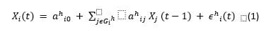
where Xi (t) is the expression (return or volatility) value for asset i at time t. The noise term is expected to be Gaussian with zero mean and a standard deviation that is estimated.
Each node in a time-series segment h receives incoming directed edges from other nodes in the parent set. The interaction parameters, the variance parameters, the number of potential parents, the location of changepoints separating the time-series segments and the number of changepoints are given (conjugate) prior distributions in a Hierarchical Bayesian model. For inference, all these quantities are sampled from the posterior distribution using RJMCMC (Reversible Jump Markov Chain Monte Carlo).
The output from this model is a sequence of different networks for each asset (child node) with one network for every segment. Using the sequence of networks for all assets (N in total), we can assess dynamics of dependence across assets. The Bayesian approach offers a natural regularization that helps maintain sparsity in the networks.
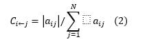
I define different measures of connectedness to estimate dependence across assets from the dynamic networks. Pairwise Connectedness is defined as
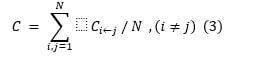
Total Connectedness is expressed as
Connectedness for Daily Return and Volatility data
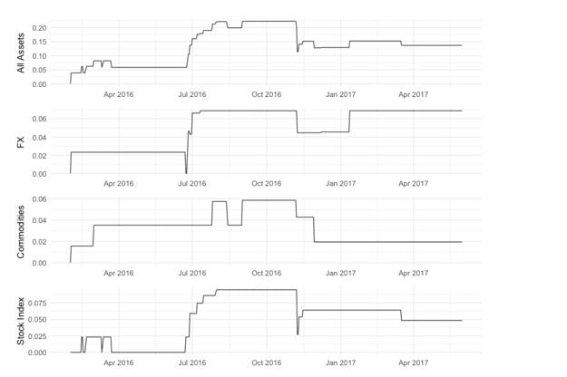
I apply the model explained in Section 2 to each of the daily returns and volatility data of 43 different assets (across global FX, Commodities and Equities) for the period ranging from February 2016 to May 2017. Our model can identify all major market shocks during this period including the BREXIT referendum, GBP flash crash and US Elections. I explore the collective sequence of networks obtained from the model and discuss the results here. Total Connectedness Index (TCI) for daily returns is shown in figure 1. The index depicts the magnitude of total connectedness across global asset returns (how closely the daily returns of assets were dependent on each other).
Figure 1: Total Connectedness Index for Daily Return Networks. Top plot shows Connectedness across all assets and the other plots show the breakdown by asset class.
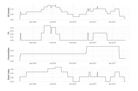
The TCI is at its maximum value towards the end of June coinciding with the BREXIT referendum period and gradually declines from mid-July as observed from the top plot (total connectedness across all assets). The other three plots in figure 1 show the breakdown of connectedness across asset classes. The increased TCI at the end of June is primarily driven by the connectedness from FX markets which increase towards the end of May leading up to the BREXIT event and drop to pre-May levels around August. Commodities connectedness was flat during this period and their returns were not impacted much by BREXIT shock. Global Equities also show an increased connectedness during this period and it lasted much longer compared to FX before falling to almost zero in October. This provides an interesting insight: the BREXIT shock correction happened immediately in FX markets as opposed to Equities where it was more gradual. Commodities had minimal correction in return connectedness during this period.
Volatility connectedness shows a slightly different picture and is shown in figure 2. The Volatility connectedness across all assets had a spike during the BREXIT period. This shows up as a sharp spike in FX connectedness while equities had a relatively gradual increase in connectedness. Volatility connectedness for Commodities painted a similar picture as its return connectedness. The increase in volatility connectedness in general lasts for a much longer period (starting from mid-June) as opposed to return connectedness which drops from mid-July.
Figure 2: Total Connectedness Index for Daily Volatility Networks. Top plot shows Connectedness across all assets and the other plots show the breakdown by asset class.
The cluster in November on Return network coincides with the lead-up to US elections and its results on 9 November 2016. This is also shown as a pronounced activity with many edges being formed in the Volatility network. The TCI reflects this with an increase in connectedness in the Return network and this increase is primarily fueled by equity markets. Donald Trump won the US Elections and this was seen as positive news in the equity markets globally as investors rapidly embraced the idea of a Republican-controlled Congress being a game changer by implementing fiscal stimulus, tax cuts and rolling back on regulations for US business, which had spillover effects into global markets. FX and Commodity return connectedness were relatively unchanged. The TCI for volatility dropped across all the charts as the overall market volatility was lower with Trump winning the election. It had the most drastic impact on equity markets with the volatility connectedness dropping by over 70%.
Booming share markets after the US election also reflected hopes of an oil production deal that eventually came to pass in late November when Opec met in Vienna. A subsequent agreement between non-Opec producers to also cut supply in December helped deliver a significant boost to crude prices. The main motivation for the deal had been the economic pain inflicted by a falling oil price on the economies of producers, notably Saudi Arabia. As Saudi Arabia was looking to line up an equity flotation of state-owned oil company Aramco, keeping the price firmly above $50 a barrel was a crucial aim. This is represented by increased connectedness in Commodities around the end of November and leading into December.
The Edge formation chart of daily returns highlights a large spike on 15 December accounting for the activity across the global assets following the Federal Reserve raising the federal funds target rate at its December meeting (13 and 14 December with hikes effective from 15 December) by a quarter of a percentage point, and further signaling three rate hikes in 2017 – an increase from its previous meeting. Supporting the central bank’s outlook, gross domestic product growth was a better-than-expected 3.5% in the third quarter, and the unemployment rate fell to 4.6% in November. The Institute for Supply Management reported the economy expanded for the 90th consecutive month in November, and the Conference Board’s consumer confidence index hit its highest level since 2001. This was shown as increased activity in our return network on the period around 15 December. This is reflected by an increase in TCI in the return network alone. Aside from the ones mentioned above, there were also other minor shocks showing up with smaller spikes in the return and volatility charts throughout the year.
Lastly, we also observe that while changes in Equity and Commodities markets connectedness usually lasted much longer, changes in FX connectedness had pronounced spikes and decayed very quickly. This indicates that the FX assets adjust to shocks more rapidly and their connectedness returns to original levels much more quickly.
Conclusion
I set out with the broad objective of developing a unified framework for identifying dynamically changing relationships across a large number of assets over a long horizon of time and across different moments of the data. I have been able to identify the change-points - points in time when the network relationships change - for each of the assets in this period as well as obtain the static network within each of the segments between two change-points. Furthermore, I have been able to corroborate the change-points with important market events and through the construction of a Total Connectedness Index, have been able to explain how the asset relationships change before and after these events, which shocks are important for each asset class and how each asset class responds to different shocks.
[1] In this article, “connectedness" refers to dependence as used in Graph Theory or Network literature.
References
Demirer, M., F.X. Diebold, L. L., and Yilmaz, K. (2017) Estimating global bank network Connectedness, Journal of Applied Econometrics 33, 1–15.
Diebold, F. and Yilmaz, K. (2014) On the network topology of variance decompositions: measuring the connectedness of financial firms, Journal of Econometrics 182, 119–134.
Lebre, S. (2007) Stochastic process analysis for genomics and dynamic bayesian networks Inference. PhD thesis, Universit ́e d‘Evry-Val-d‘Essonne, France.
Lebre, S., Becq, J., Devaux, F., Lelandais, G., and Stumpf, M. (2010) Statistical inference of the time-varying structure of gene-regulation networks, BMC Systems Biology 4,130.


